Timing plan · 90 minutes
- 0–6Recap of the five budgets; today's question: what has already been lost before the model sees the data?
- 6–16The sensing chain; the sensors you will meet; signals in time and frequency (Fig 2.2).
- 16–30Sampling and aliasing, with the interactive explorer; quantization, SQNR and ENOB.
- 30–40Noise and filtering (moving average versus median); sampling rate and resolution as energy decisions.
- 40–45Datasets, labels, normalisation, and leakage.
- 45–52Break.
- 52–58Windows and segmentation (Fig 2.9); three questions to ask of any representation.
- 58–74Time-domain features; the STFT and its resolution trade-off; mel and MFCC derived on the board.
- 74–84IMU and image features; feature selection; PCA, LDA, and what t-SNE is for.
- 84–90Takeaway; preview of Session 3.
In one sentence
Every stage between the physical world and the model — transducer, filter, sampler, quantizer, window, transform — throws information away, and the engineering question is always whether it threw away the part the model needed, at a price the budget can pay.
2.1The chain, and what each stage costs
Analog versus digital sensors. An analog sensor delivers a continuous voltage and requires the whole chain above; you own the anti-alias filter, the reference, and the noise budget. A digital sensor (an I²S MEMS microphone, an I²C IMU) has the converter on-die and hands you samples over a bus — convenient, but the conversion decisions have been made for you and are visible only in the datasheet. The important point is that "digital sensor" does not mean "no signal processing"; it means the processing happened somewhere you cannot change, so you must read its specification: sensitivity, acoustic overload point, SNR, and the on-chip decimation filter's group delay.
2.2The sensors you will meet
A sensor (more precisely, a transducer plus its conditioning electronics) converts a physical quantity — pressure, acceleration, light, voltage across skin — into an electrical signal. Most sensors used in embedded ML today are MEMS devices (micro-electro-mechanical systems): microscopic mechanical structures etched in silicon, packaged with their own amplifier and often their own analog-to-digital converter, which deliver digital samples over a serial bus. For the ML engineer, four properties of a sensor matter more than its physics: its sampling rate, its resolution and noise floor, its interface, and its power draw while sampling.
| Sensor | Measures | Typical rate | Bits | Interface | Active power |
|---|---|---|---|---|---|
| MEMS microphone | sound pressure | 16–48 kHz | 16–24 | PDM or I²S | ≈ 0.3–1 mW |
| Accelerometer | linear acceleration, 3 axes | 10 Hz–6.4 kHz | 12–16 | I²C / SPI | ≈ 5–200 µW |
| Gyroscope | angular rate, 3 axes | 25 Hz–6.4 kHz | 16 | I²C / SPI | ≈ 1–3 mW |
| PPG (optical heart rate) | blood-volume changes | 25–500 Hz | 16–20 | I²C | ≈ 0.1–2 mW (LED) |
| ECG front end | cardiac potential | 125–1000 Hz | 12–24 | SPI / ADC | ≈ 10–300 µW |
| Environmental | temperature, humidity, gas | 0.01–10 Hz | 12–24 | I²C | µW (gas: mW, heated) |
| Low-res camera | light intensity, 2-D | 1–30 fps | 8 per pixel | DCMI / SPI / MIPI | ≈ 1–100 mW |
| mmWave radar | range, velocity, angle | frames at 10–100 Hz | 12–16 | SPI / LVDS | ≈ 0.1–1 W (duty-cycled) |
Table 2.1 — Sensors in embedded ML. Order-of-magnitude ranges across common parts; the active-power column is the sensor alone. Note that a gyroscope costs one to two orders of magnitude more power than an accelerometer — a classic reason to infer orientation from the accelerometer alone when the application allows it.
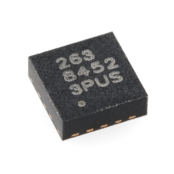
Photo: Wikimedia Commons
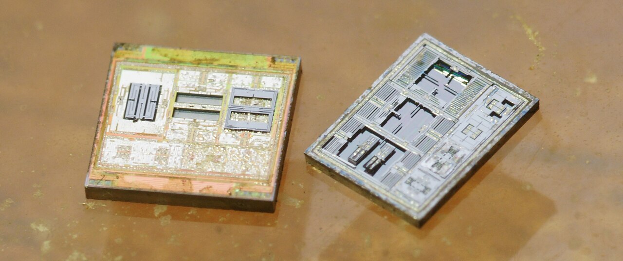
Photo: Wikimedia Commons
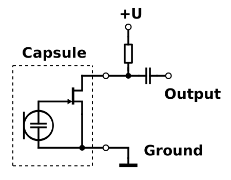
Photo: Wikimedia Commons
Two practical lessons recur. First, many sensors can do part of the processing themselves: modern IMUs contain FIFO buffers, step counters and even small programmable state machines or decision-tree engines, so the main MCU can sleep until something interesting happens — the cascade of Session 1 implemented inside the sensor. Second, the sensor's configuration (range, rate, filter) is part of the model's input specification: a classifier trained on data captured at ±4 g and 100 Hz will fail silently on a device configured for ±16 g and 50 Hz. Record the configuration with the data.
2.3Signals in time and frequency — a primer
A signal here is a sequence of numbers indexed by time, x[n] = x(n·Ts), where Ts is the sampling interval and fs = 1/Ts the sampling rate. You can describe it in two equivalent ways: by its values over time, or by how much of each frequency it contains. The second description is the key to almost everything in this session.
The bridge is Fourier's observation that any reasonable signal is a sum of sinusoids. A sinusoid A·sin(2π f t + φ) has three properties: amplitude A, frequency f (cycles per second, Hz) and phase φ. The spectrum of a signal lists the amplitude (and phase) of each frequency it contains.
Foundations · the discrete Fourier transform in five lines
For a block of N samples, the discrete Fourier transform (DFT) computes N complex numbers
Each X[k] measures how strongly the block correlates with a sinusoid at frequency fk = k · fs/N; its magnitude |X[k]| is the amplitude, its angle the phase. Three facts follow directly. The frequency resolution is fs/N: a longer block resolves finer frequency differences. For a real signal only the first N/2 + 1 bins are independent; the highest representable frequency is fs/2. And the fast Fourier transform (FFT) computes all N bins in about N·log₂N operations instead of N² — for N = 512, on the order of 4 600 complex operations (2 304 radix-2 butterflies) instead of N² ≈ 262 000 complex multiplications, which is why spectral features are affordable on a microcontroller at all.
Foundations · convolution, filtering and the frequency domain
A linear, time-invariant filter is fully described by its impulse response h[n]: its output is the convolution y[n] = Σₖ h[k]·x[n−k], a sliding weighted sum — the moving average is the simplest example. The convolution theorem says that convolution in time is multiplication in frequency: Y(f) = H(f)·X(f). A low-pass filter is therefore a multiplication of the spectrum by a function that is near 1 at low frequencies and near 0 at high ones. The theorem also works the other way round: multiplying two signals in time convolves their spectra. Sampling is exactly such a multiplication — the continuous signal times a train of impulses spaced Ts apart — and the spectrum of an impulse train is itself an impulse train spaced fs apart. Convolving with it makes copies of the signal's spectrum at every multiple of fs, which is the picture behind the sampling theorem and aliasing in the next section. (The same word, convolution, names the core layer of CNNs in Session 3: there too it is a sliding weighted sum, with learned weights.)
Why should an ML engineer care? Because most physical processes are easier to recognise in frequency than in time. A bearing fault produces vibration at a characteristic frequency; a spoken vowel is a pattern of resonances; walking is a periodic motion at about 2 Hz. And because the operations of the sensing chain — filtering, sampling, windowing — have simple descriptions in the frequency domain and complicated ones in time.
2.4Sampling and aliasing, stated precisely
Sampling theorem. A signal whose spectrum is zero outside |f| < B is completely determined by samples taken at rate fs > 2B, and is reconstructed by sinc interpolation. Sampling in time multiplies by an impulse train, which convolves the spectrum with an impulse train of spacing fs: the spectrum is periodically replicated. If fs < 2B, adjacent replicas overlap and add. That overlap is aliasing, and it is an addition, not an occlusion — which is why it is irreversible.
A component at frequency f appears after sampling at the folded frequency
so a 30 kHz interferer sampled at 16 kHz lands at 2 kHz, squarely inside a speech band, and is now indistinguishable from real speech energy.
Design consequence students routinely miss
A brick-wall analog filter does not exist. Real filters have a transition band, so practical designs sample at 2.2–2.5× the highest wanted frequency and let the filter roll off across the guard band, or oversample heavily and do the sharp filtering digitally (§2.7). "Sample at exactly 2B" is a theorem, not a design.
2.5Quantization noise, SQNR and ENOB depth
Derivation — the 6.02 N + 1.76 dB rule
An N-bit converter with full-scale range VFS has step size q = VFS/2N. Model the rounding error e as uniformly distributed on [−q/2, q/2] and independent of the signal — a good approximation when the signal is busy relative to q. Its power is
A full-scale sinusoid of amplitude VFS/2 has power VFS²/8. Therefore
Each additional bit buys about 6 dB. Two corollaries matter in practice:
- Headroom is expensive. If your signal only ever reaches −20 dBFS, you have thrown away more than three bits. Gain staging is therefore part of the ML pipeline, not merely electronics.
- Nominal bits ≠ effective bits. Datasheets quote ENOB, derived from measured SINAD by inverting the formula: ENOB = (SINAD − 1.76)/6.02. A "16-bit" ADC on a noisy PCB may deliver 11–12 ENOB. Design against ENOB.
Dither. The independence assumption fails for very small or very periodic signals, where the error becomes correlated with the signal and appears as harmonic distortion — audible as tones rather than hiss. Adding a small amount of noise (about 1 LSB rms) before quantization decorrelates the error, trading a slightly higher noise floor for the removal of structured artefacts. This matters for embedded audio because structured artefacts are exactly what a spectrogram-based classifier will latch onto.
Averaging and oversampling. Averaging M independent samples of a stationary signal reduces noise power by M, i.e. SNR improves by 10 log₁₀ M dB — about 3 dB per doubling, or half a bit. Getting one extra effective bit therefore costs 4× the samples. This is the exchange rate between analog quality and digital effort, and it is the basis of sigma-delta converters, which deliberately oversample by 64–256× and shape the quantization noise out of the band of interest.
2.6Noise budget and filtering
Sources, in the order they usually dominate on a real board: power-supply and switching noise coupled through the reference; electromagnetic interference at mains frequency and its harmonics; thermal (Johnson) noise, white, proportional to √(4kTRB); 1/f (flicker) noise, dominant at low frequencies and the reason DC-coupled measurements are hard; quantization noise, usually the smallest of the five. Note the ordering: students are taught quantization noise and then find that it is rarely the limiting term.
Foundations · three converter architectures, and what each implies for you
| Architecture | How it works | Typical | Consequence for an ML pipeline |
|---|---|---|---|
| SAR (successive approximation) | Binary search: one comparison per bit against a DAC | 8–18 bit, kSPS–MSPS | The MCU default. One conversion per trigger, low latency, easy to interleave across channels — good for IMU and general sensing. |
| Sigma–delta (ΣΔ) | 1-bit modulator at 64–256× oversampling, then a digital decimation filter shapes the noise out of band | 16–24 bit, kSPS | Audio and precision sensing. Buys resolution with digital effort instead of analog precision — but its decimation filter adds group delay, which matters if you are timestamping events or fusing sensors. |
| Flash / pipeline | 2N−1 comparators in parallel, or a pipeline of small stages | 6–14 bit, MSPS–GSPS | Radar, ultrasound, RF. Fast and power-hungry; you will be bandwidth-limited downstream long before the converter is the problem. |
Table 2.2 — Converter architectures. Notice the pattern: each buys resolution with a different currency — comparisons (SAR), time and digital filtering (ΣΔ), or silicon area and power (flash). That is the same trade structure you will meet again in Session 4, one abstraction level up.
Foundations · the decibel, and why everything here is logarithmic
A decibel is a ratio of powers on a log scale: 10 log₁₀(P₁/P₀), or equivalently 20 log₁₀(A₁/A₀) for amplitudes, since power goes as amplitude squared. Three numbers are worth internalising:
- 3 dB = a factor of 2 in power. Averaging two independent samples, or doubling the oversampling ratio, buys you exactly this.
- 6 dB = a factor of 2 in amplitude — one bit. Hence §2.5's rule.
- 20 dB = a factor of 10 in amplitude, 100 in power.
The reason the whole signal chain is measured this way is that its stages multiply: a sensor's sensitivity, an amplifier's gain and a converter's full-scale range compose by multiplication, and logarithms turn that into addition. It is also how a noise budget is assembled — powers of independent noise sources add, so the total is √(σ₁² + σ₂² + …) and one source 10 dB above the rest simply is the answer.
Watch the reference, which is where mistakes are most common: dBFS is relative to the converter's full scale and is therefore never positive; dBSPL is relative to 20 µPa of acoustic pressure; dBA is dBSPL after a perceptual weighting curve. A microphone datasheet quoting “65 dB SNR” means SNR at 94 dBSPL, A-weighted — a different quantity from the SQNR of the converter behind it.
FIR versus IIR on an embedded target
| Property | FIR | IIR |
|---|---|---|
| Cost per output sample | M MACs (M taps) | ≈ 2·order MACs (biquads) |
| State memory | M words | 2 words per biquad |
| Phase | Exactly linear if symmetric | Non-linear; group delay varies |
| Stability | Always stable | Can oscillate; poles must stay inside the unit circle |
| Fixed-point pathologies | Overflow in the accumulator | Coefficient quantization moves poles; limit cycles; needs cascaded biquads and careful scaling |
| Typical use | Decimation, matched filtering, anything where phase matters | Cheap band-limiting, DC blocking, envelope tracking |
Table 2.3 — Choosing a filter structure. For a given magnitude specification an IIR filter is typically an order of magnitude cheaper than an FIR one; you pay in phase linearity and numerical fragility.
The moving average is an FIR filter with impulse response 1/M over M taps, and its frequency response is a Dirichlet (periodic sinc) kernel: a wide main lobe and first sidelobe only about 13 dB down. It is cheap and it is a poor low-pass filter, and it is worth looking at its magnitude response once, to stop treating "smoothing" as free. The moving median, by contrast, is non-linear: it removes impulsive outliers without smearing edges, has no frequency response at all, and costs a sort or a running-order-statistic structure — often the right choice for IMU spike removal and the wrong choice for anything you will later transform.
Fixed-point implementation. On MCUs without an FPU, filters run in Q-format fixed point. Three rules: accumulate in a wider type than you multiply in (Q15 × Q15 → Q30 in a 32-bit accumulator); scale coefficients so intermediate results cannot overflow, or use saturating arithmetic; and implement high-order IIR filters as cascaded second-order sections, because direct-form high-order implementations are numerically catastrophic. CMSIS-DSP's biquad functions exist for exactly these reasons.
2.7Sampling rate and resolution are energy decisions
Sampling rate propagates multiplicatively through the whole downstream cost: ADC energy per conversion × rate, filter MACs per sample × rate, frames per second × feature cost, inferences per second × model cost. Halving fs where the application allows it is usually the single largest energy saving available, and it is free of accuracy loss if the discarded band carries no class-discriminative information — a claim that should be tested empirically, not assumed. For keyword spotting, 16 kHz is conventional and 8 kHz is often sufficient; for bearing-fault detection the diagnostic energy may sit above 10 kHz and the same reasoning gives the opposite answer.
Oversample-and-decimate is the standard escape from expensive analog design: sample at R·fs with a gentle analog filter, apply a sharp digital low-pass, then keep every R-th sample. Two efficiency notes for embedded targets: the decimating filter should be implemented as a polyphase structure so it only computes the outputs that survive (an R× saving), and cascaded integrator-comb (CIC) filters achieve large decimation ratios with no multipliers at all, which is why they appear inside PDM microphone front ends.
2.8Datasets, labels and preprocessing
The signal chain delivers samples; a learning algorithm needs a dataset: many examples, each paired with a label, that represent the conditions the device will meet in the field. For embedded sensing problems the dataset is usually the most expensive and least reusable part of the project, and the most common cause of disappointing field performance.
Collection and labelling
- Coverage beats volume. Record across the variation the device will see: different users, mounting positions, devices of the same model (sensor gains differ), environments, background activities. A thousand recordings from one person are worth less than a hundred from fifty.
- Label granularity is a design decision. A recording may be labelled as a whole ("this minute contains a fall"), per window, or with exact event boundaries. Coarse labels are cheap; fine labels are needed to train detectors with accurate onsets. Weakly labelled learning is an active research area precisely because fine labels are so expensive.
- Rare events and class imbalance. The events you care about — faults, falls, arrhythmias, a wake word — are usually rare. Plan for it: collect targeted examples, use a background ("none of the above") class that is genuinely diverse, and evaluate with metrics that are not fooled by imbalance (Session 3).
- Public datasets. Speech Commands (keyword spotting), ESC-50 and UrbanSound8K (environmental audio), UCI-HAR and PAMAP2 (activity recognition), MIT-BIH (arrhythmia), MIMII and ToyADMOS (machine sound anomalies), Visual Wake Words (person detection). They are ideal for comparison and teaching, and dangerous as a proxy for your own deployment conditions.
Cleaning and preprocessing
Before features, the raw data usually needs: synchronisation of streams sampled by different clocks; resampling to the rate the deployed device will use; handling of gaps (dropped packets, sensor saturation) — by interpolation, masking or discarding windows; outlier and artefact removal (the median filter above); and calibration (offset and gain per sensor). Every one of these steps must also exist, identically, in the firmware — a discrepancy between the training pipeline in Python and the deployed pipeline in C is one of the most common causes of embedded models that "worked in the notebook".
Normalisation
Most learning algorithms assume features on comparable scales. Standardisation (z-scoring) subtracts the training-set mean and divides by the training-set standard deviation of each feature; min–max scaling maps the training range to [0, 1]. Decision trees are indifferent to scaling; neural networks, SVMs, k-nearest neighbours and anything trained by gradient descent are not (the reason is visible in the gradient-descent figure of Session 3). On an embedded device the normalisation is two constants per feature, applied in the firmware — and, conveniently, it can be folded into the first layer's weights and the quantization parameters (Session 3), so it often costs nothing at run time.
Augmentation
Data augmentation creates plausible new training examples from existing ones: time shifts, added background noise at various signal-to-noise ratios, gain changes and room reverberation for audio; small rotations of the sensor frame, time warping and amplitude scaling for IMU data. It is free at inference time and often the cheapest accuracy improvement available to a small model, because small models are more sensitive to the gap between training and field conditions. SpecAugment-style masking of time and frequency bands is standard for spectrogram inputs.
Common misconception
"We split the data randomly into training and test sets, so the test accuracy is honest." Not for windowed sensor data. Overlapping windows cut from the same recording are near-copies; a random split puts copies on both sides, and the test score measures memorisation of that recording. The same holds, less obviously, for windows from the same person or the same machine. Split by subject, device or session — Session 3 shows the picture. Fit normalisation constants and feature selection on the training portion only, for the same reason.
2.9Framing, windowing and segmentation
Models consume frames, not streams. A frame length L with hop H gives an overlap of 1 − H/L and a frame rate of fs/H. Three consequences: the frame rate sets the inference rate and therefore the energy; the frame length sets the lowest frequency that can be resolved (fs/L); and the hop sets the temporal precision of an event's onset. Overlap is not free — 50 % overlap doubles the number of inferences — so on an energy-limited device it is a parameter to be justified, not a default. §2.12 takes this up properly with the time–frequency uncertainty relation.
For event-like data the fixed sliding window is not the only option. Event-triggered segmentation starts a window when a cheap detector (an energy threshold, a step detector in the IMU) fires, which aligns windows with the events and saves energy between them. Labels must be assigned per window — by majority vote over the samples in it, by "any event present", or by the label at the window centre — and that choice changes what the model learns about onsets. Write it down.
2.10Three questions to ask of any representation
- What does it discard, and is the discarded part class-discriminative? Mel warping discards fine high-frequency resolution — irrelevant for speech, potentially fatal for ultrasonic fault detection.
- What invariances does it build in? The magnitude spectrogram discards phase and thereby buys invariance to time shift within a frame. If your task depends on inter-channel phase (direction of arrival), you have just deleted the signal.
- What does it cost, and against what baseline? Compare the front end's MACs and memory with the model's. If the front end costs 40 % of the budget, a learned front end operating on raw samples may be cheaper overall.
2.11Time-domain features
The cheapest features are computed directly on the samples of a window, with one pass and no transform. For a window x[0…N−1]:
plus higher-order statistics (skewness, kurtosis), percentiles, and counts of threshold crossings. Each costs O(N) operations — tens of microseconds on an MCU for a typical window — and many can be updated incrementally as each sample arrives, so the window never needs to be stored at all.
These features are what the first stage of a cascade is built from: a voice-activity detector, a "something is moving" trigger for an IMU, or an "unusual vibration energy" alarm. They are also more powerful than they look for slowly varying physical signals, and a sensible baseline for any new task: if a decision tree on ten time-domain statistics already reaches the target accuracy, the project does not need a neural network.
2.12The short-time Fourier transform depth
The Fourier transform assumes stationarity over its whole support; speech, vibration and gesture signals are not stationary. The STFT applies the transform to short windowed segments in which stationarity is approximately true:
with window w of length L and hop H. The spectrogram is |X[m,k]|².
Windows and leakage
Truncating with a rectangular window multiplies in time, hence convolves in frequency with a Dirichlet kernel whose first sidelobe is only ≈13 dB down. A strong component therefore leaks into neighbouring bins and can bury a weak one. Tapered windows trade main-lobe width (resolution) for sidelobe suppression (dynamic range):
| Window | Main lobe width | Peak sidelobe | Use when |
|---|---|---|---|
| Rectangular | 2 bins | −13 dB | Transient onsets; never for spectral estimation |
| Hann | 4 bins | −31 dB | Default for speech/audio; sums to unity at 50 % overlap |
| Hamming | 4 bins | −43 dB | Classic speech front ends |
| Blackman–Harris | 8 bins | −92 dB | Large dynamic range, e.g. vibration with a dominant shaft tone |
Table 2.4 — Window trade-offs. Widths are approximate, in units of the DFT bin spacing fs/L. Choosing a window is choosing where on the resolution/dynamic-range curve your task sits.
The uncertainty relation, and what it means operationally
Frequency resolution is Δf ≈ fs/L and time resolution is Δt = L/fs, so Δt·Δf ≈ 1 — a bound, not a tuning knob (for a Gaussian window the exact statement is σtσf ≥ 1/4π). You cannot resolve a 20 ms transient and a 10 Hz frequency difference in the same analysis. Increasing overlap increases the frame rate and thus the smoothness of the picture, but it does not improve Δt; the smearing is set by L. Students conflate these constantly.
2.13From spectrogram to mel and MFCC
Human auditory frequency resolution is approximately logarithmic above ~1 kHz. The mel scale encodes this; the most commonly used form is
A mel filterbank places B triangular filters equally spaced on the mel axis and applies them to the power spectrum, reducing, say, 257 FFT bins to 40 mel bands — a 6× dimensionality reduction that is nearly free of task-relevant information for speech. The classical MFCC pipeline then continues:
Why each step exists. Pre-emphasis (y[n] = x[n] − αx[n−1], α ≈ 0.97) flattens the roughly −6 dB/octave spectral tilt of voiced speech so that high-frequency detail is not numerically swamped. Log compression converts multiplicative channel effects into additive offsets, which is what makes cepstral mean normalisation a valid channel-compensation method. DCT-II approximates the Karhunen–Loève transform for this class of signals, decorrelating the coefficients; keeping the first 12–13 discards the fine spectral detail that encodes pitch. Liftering rescales coefficients so their dynamic ranges are comparable.
Deltas. First and second time derivatives (Δ, ΔΔ), computed by regression over ±2 frames, add dynamic information to an otherwise static frame representation. For a CNN or an RNN with temporal context they are largely redundant, since the model can compute them; for an SVM or GMM over single frames they are essential. This is a good illustration of the general rule that feature engineering compensates for what the model class cannot learn.
2.14IMU and image features
IMU (accelerometer / gyroscope). A well-tested feature set for human-activity recognition, per axis per window: mean, standard deviation, min, max, interquartile range, root-mean-square, skewness, kurtosis, zero-crossing rate, signal-magnitude area, correlation between axes, and the norm √(ax²+ay²+az²), which is rotation-invariant and therefore robust to how the device is worn. Frequency-domain additions: dominant frequency, spectral entropy (flatness of the spectrum, distinguishing periodic walking from aperiodic fidgeting), band energies, and autocorrelation peak lag for cadence. Jerk (the derivative of acceleration) separates smooth from abrupt motions. Note that on a 50 Hz IMU a 2.56 s window is 128 samples — an FFT of that size is trivial, so the choice of time- versus frequency-domain features is about statistics, not cost.
Images. Handcrafted descriptors — edges, corners, colour histograms, HOG, LBP, Haar features over an integral image — were the state of the art before 2012 and remain competitive under extreme constraints, where the alternative model would have to be very small. In current practice a learned front end (a few convolutional layers of a MobileNet-class network) dominates whenever the compute exists, and the interesting question for this course is exactly where the crossover sits on a given device.
| Front end | Approx. cost / frame | Output dim | Notes |
|---|---|---|---|
| Time-domain statistics, 3-axis IMU, 128 samples | ~10³ ops | ~30 | Negligible; runs in the sensor ISR |
| 512-point real FFT | ~10⁴ MACs | 257 | CMSIS-DSP; radix-2/4 |
| 40-band log-mel from 512-point FFT | ~1.5 × 10⁴ MACs | 40 | Filterbank is sparse; log dominates if done naively |
| 13 MFCC + Δ + ΔΔ | ~1.6 × 10⁴ MACs | 39 | Adds a small DCT |
| Small DS-CNN over a 49×10 MFCC map | ~2.7 × 10⁶ MACs | — | Model ≈ 4× the front end over a full second (49 frames ≈ 7 × 10⁵ MACs) |
Table 2.5 — Order-of-magnitude front-end costs, for building the habit of comparing front end against model. The comparison flips for very small models and for high sample rates: measure, do not assume.
Common misconception
“Feature extraction is preprocessing, so it is free.” On a Cortex-M4F running a 40 kB keyword spotter at 16 kHz with 50 % overlap, the FFT-plus-mel front end can consume a third of the cycle budget and more than a third of the energy, because it runs on every frame while the classifier may run on a subsample of them. Profile the front end and the model separately, and count the front end's cost against the same budget as the model's.
2.15Feature selection depth
Three families, in increasing cost and decreasing generality:
- Filter methods score each feature against the label independently of any model. Pearson correlation ρ = cov(X,Y)/(σXσY) captures only linear dependence and will assign zero to a perfect quadratic relationship. Mutual information, I(X;Y) = H(Y) − H(Y|X), captures any dependence but must be estimated — typically by k-nearest-neighbour estimators — and estimation error grows quickly with dimension. Filters are cheap and ignore redundancy: two perfectly correlated informative features both score highly and both get selected.
Foundations · entropy and mutual information in three lines
Entropy is the average number of nats (or bits, with log₂) needed to describe a draw from a distribution: H(Y) = −Σ p(y) log p(y). A fair coin has H = 1 bit; a coin that always lands heads has H = 0 — nothing to communicate.
Conditional entropy H(Y|X) is what remains uncertain about Y once you know X. Mutual information is the difference: I(X;Y) = H(Y) − H(Y|X) — literally how many bits knowing X saves you. It is zero exactly when the variables are independent, symmetric in its arguments, and invariant to any invertible transformation of either variable, which is why it does not care whether the relationship is a line, a parabola or a circle.
The price is estimation. Entropy of a continuous variable has to be estimated from samples — usually by binning or by nearest-neighbour distances — and the estimator's variance grows sharply with dimension. That is the honest reason Pearson correlation survives in practice despite being obviously weaker: it has a closed form and no hyperparameters.
- Wrapper methods search over subsets using the model itself as the scoring function. Recursive feature elimination fits the model, ranks features by an importance measure, removes the weakest, and repeats. Expensive but accounts for interactions and redundancy.
- Embedded methods select during fitting. Lasso minimises ‖y − Xβ‖² + λ‖β‖₁; the L1 penalty's corner geometry drives coefficients exactly to zero, so the fit and the selection are one problem. Tree ensembles give impurity- or permutation-based importances — prefer permutation importance, since impurity importance is biased toward high-cardinality features.
The hygiene rule that decides whether a result is valid
Feature selection is part of the model, so it must happen inside each cross-validation fold, using only that fold's training data. Selecting features on the full dataset and then cross-validating the classifier leaks label information and produces optimistic estimates — routinely several accuracy points, and much more when the number of features exceeds the number of samples. The same applies to normalisation statistics, PCA bases, and class-balancing.
2.16Dimensionality reduction
PCA in one derivation
Centre the data, X̃ = X − μ. Seek the unit direction w maximising the projected variance wTΣw subject to wTw = 1, where Σ = X̃TX̃/(n−1). The Lagrangian gives Σw = λw: the optimal directions are the eigenvectors of the covariance matrix, and the variance captured by each is its eigenvalue. Keep the top d so that Σi≤dλi / Σiλi reaches your threshold. In practice compute it by SVD of X̃ rather than by forming Σ, which squares the condition number.
On device PCA is just a matrix multiply by a stored D×d matrix — cheap at inference, but the matrix itself occupies flash, which can exceed what the reduction saves. Always compare D·d stored weights against the parameters saved downstream.
LDA is supervised: it maximises the Fisher criterion wTSBw / wTSWw, the ratio of between-class to within-class scatter. Its output is capped at C−1 dimensions for C classes — a hard structural limit worth remembering — and it assumes roughly Gaussian, equal-covariance classes.
t-SNE and UMAP are non-linear neighbour-embedding methods for visualisation. Both optimise a notion of local neighbourhood preservation; both distort global distances; t-SNE has no natural out-of-sample extension at all. They are excellent for inspecting whether your classes separate before you spend a week training, and they must never appear in a deployed pipeline. Beware of reading cluster sizes and inter-cluster distances in a t-SNE plot: neither is meaningful.
Random projection deserves more attention than it gets in embedded work. The Johnson–Lindenstrauss lemma guarantees that projecting onto O(log n / ε²) random directions preserves all pairwise distances to within 1±ε. With a sparse or ±1 projection matrix generated from a stored seed, the projection costs additions only and needs no stored matrix — an unusually good fit for a microcontroller.
PCA versus LDA, and t-SNE, on pictures
The two figures below make the comparison of this section concrete. In the first, the direction of greatest variance is exactly the wrong one to keep for classification; LDA, which uses the labels, finds the one that separates the classes. Both are a fixed matrix multiply at inference time, with parameters estimated on the training split only.
The second figure shows the same contrast between a linear projection and a non-linear embedding on real data. Use the t-SNE view to understand a dataset — whether classes form clusters, which examples are mislabelled, whether one subject's recordings sit apart from the rest — and never as a stage of the deployed pipeline.
If you remember one thing from Session 2
Decide what your model must be able to distinguish, then work backwards: the bandwidth sets the sampling rate, the dynamic range sets the bits, the event duration sets the window, and the cheapest representation that keeps the distinguishing information is the right one. Anything lost before the model is lost for good — and anything kept that the model does not need is paid for in every inference.
Before Session 3
- Y. Zhang, N. Suda, L. Lai, V. Chandra, "Hello Edge: Keyword Spotting on Microcontrollers," 2017. arXiv:1711.07128.A complete embedded pipeline — MFCC front end, several model families, memory and operation budgets — in twelve pages. Session 3 uses its numbers.
- If you have no ML background: work through the primer sections at the start of Session 3 before the lecture.
Discussion questions
- A colleague proposes to sample an accelerometer at 25 Hz "because human motion is below 10 Hz". What do you need to know about the sensor's internal filter before agreeing?
- Name a task for which discarding phase (taking the magnitude spectrogram) destroys the information the model needs.
- When is a learned front end (a 1-D convolution on raw samples) likely to be cheaper overall than an FFT plus mel filterbank?
- Your test accuracy drops from 97 % to 81 % when you change from a random split to a subject-wise split. What have you learned, and what do you report?
Exercises
- A 12-bit ADC digitises a sensor whose useful signal spans 20 % of the full-scale range. What is the effective SQNR for that signal, and how many bits are effectively "used"?
- Compute the number of frames, the frequency resolution and the output size of a 512-point STFT with hop 160 on one second of 16 kHz audio. How do they change with a 1024-point frame?
- An IMU samples at 50 Hz. You need to recognise gestures lasting 0.6–1.5 s with a decision latency below 1 s. Propose window length, hop and three features, and estimate the compute per second.
- Derive the cost in MACs of computing 40 log-mel energies from a 512-point power spectrum when the filterbank is stored sparsely.
Further reading
- A. V. Oppenheim and R. W. Schafer, Discrete-Time Signal Processing, 3rd ed., Pearson, 2010.The reference for sampling, filtering and the DFT.
- P. Warden, "Speech Commands," 2018. arXiv:1804.03209.Dataset design for embedded audio.
- D. S. Park et al., "SpecAugment," Interspeech 2019. arXiv:1904.08779.The standard augmentation for spectrogram inputs.
- Q. Kong et al., "PANNs: Large-Scale Pretrained Audio Neural Networks for Audio Pattern Recognition," IEEE/ACM TASLP 2020. arXiv:1912.10211.How far learned audio representations go when compute is plentiful — the opposite end of the spectrum from this course.